Understanding Neural Network Activation Functions

Activation functions might just be the unsung heroes of neural networks. Without them, you'd be stuck with linear models, severely limiting the power of your network and its ability to learn and represent complex patterns in our data. If you’re aiming to build a robust neural network, understanding these functions is key; let's explore their unique characteristics and optimal use cases.

What are Activation Functions?

Simply put, activation functions decide the output of a neuron based on its input. They transform the weighted sum of inputs (which have been turned into some numberical representation) into an output signal that the next layer can use. As you can imagine, your choice here can greatly influence your network's learning and performance.

Common Activation Functions

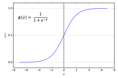
1. Sigmoid

• Range: (0, 1)
• Equation: σ(x) = 1 / (1 + e^(-x))
• Impact: Once a favorite for its simplicity and probability-friendly outputs, Sigmoid has fallen out of favor for hidden layers due to its tendency to squash gradients, especially for large positive or negative inputs.

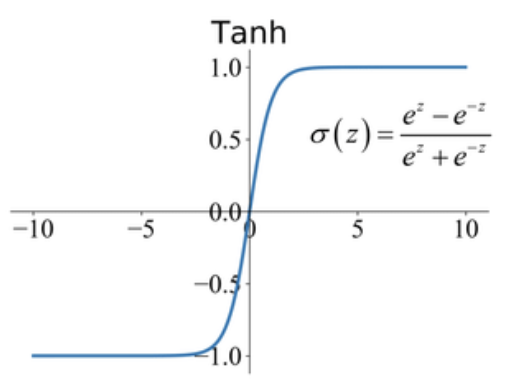
2. Tanh

• Range: (-1, 1)
• Equation: tanh(x) = (2 / (1 + e^(-2x))) - 1
• Impact: Zero-centered and preferred over Sigmoid in certain cases, Tanh still struggles with the vanishing gradient problem when inputs are extreme.

3. ReLU

• Range: [0, ∞)
• Equation: f(x) = max(0, x)
• Impact: ReLU brought a breath of fresh air by tackling the vanishing gradient issue, keeping gradients intact for positive inputs — though it can sometimes cause "dead neurons."

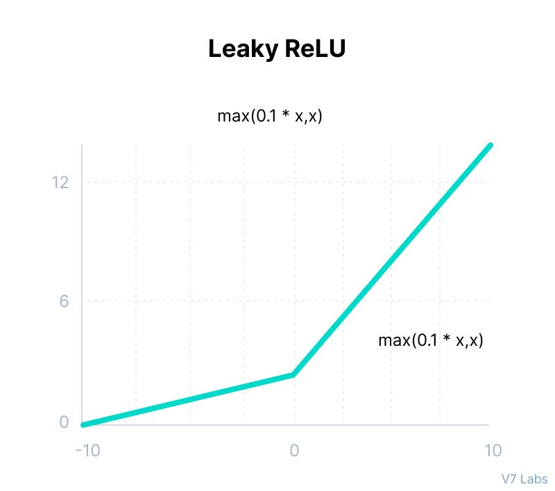
4. Leaky ReLU

• Range: (-∞, ∞)
• Equation: f(x) = max(0.01x, x)
• Impact: By allowing a small gradient for negative inputs, Leaky ReLU aims to solve the dead neuron problem of plain ReLU. You’ll see it quite a bit in practice.

5. Parametric ReLU (PReLU)

• Range: (-∞, ∞)
• Equation: f(x) = max(αx, x), where α is a learned parameter
• Impact: PReLU learns the slope of the negative part during training, offering flexibility and potential performance boosts in tricky models.

6. ELU

• Range: (-1, ∞)
• Equation:
  • f(x) = x for x > 0
  • f(x) = α(e^x - 1) for x ≤ 0
• Impact: ELU brings smoother negative values, reducing bias shifts and speeding up learning compared to other ReLU variants.

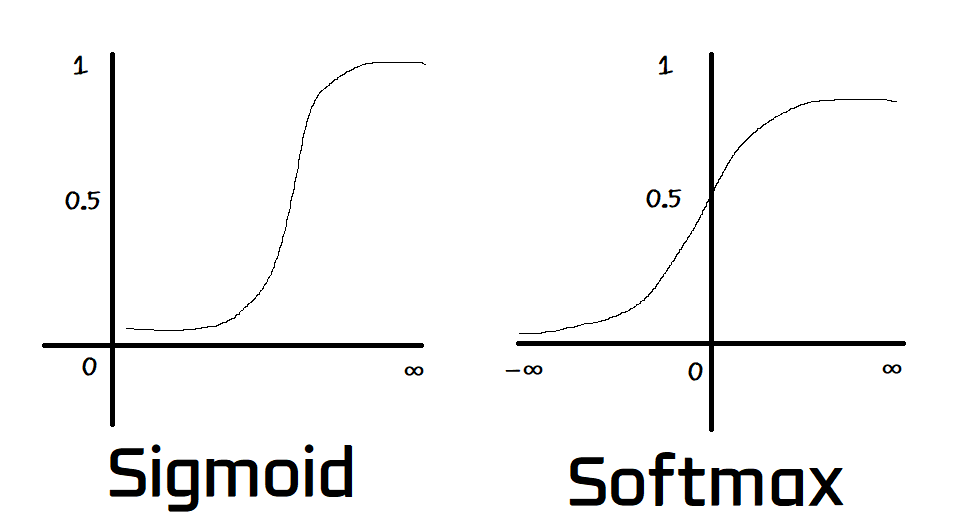
7. Softmax

• Range: (0, 1) for each output, sum of outputs = 1
• Equation: f(x_i) = e^(x_i) / Σ(e^(x_j)) for j=1 to N
• Impact: Perfect for multi-class classification, Softmax outputs probabilities that sum to 1, making it a "smart normalizer" that highlights larger values.

8. Swish

• Range: (-∞, ∞)
• Equation: f(x) = x * σ(x)
• Impact: Swish is the new kid on the block, showing promise in deep networks with its smooth gradients, sometimes outperforming ReLU.

Choosing the Right Activation Function

Choosing the right activation function is all about context. Here’s a quick guide:

Output Layer

• Binary Classification: Sigmoid
• Multi-Class Classification: Softmax
• Unbounded Regression: Linear
• Bounded Regression: Tanh

Hidden Layer

• Modern Networks: ReLU or Leaky ReLU
• Dead Neuron Issues: ELU or Swish
• Training Stability: PReLU
• RNNs/LSTMs: Traditionally Tanh, but modern networks may benefit from Leaky ReLU

Key Considerations

1. Efficiency: ReLU variants are computationally efficient.
2. Network Depth: Deeper networks need functions that prevent vanishing gradients.
3. Stability: ELU and Leaky ReLU offer stable training.
4. Task Specificity: Match your output layer activation to your task.

Conclusion

Activation functions are the backbone of neural network architectures, impacting how well your model learns and performs. While ReLU and its variants are often the go-to, don’t shy away from experimenting with other options. A well-chosen activation function can make all the difference in the world, and the only way to know which one is right for your model is to try them out.