It's Everywhere: Pip Install Torch

If you've been exploring the open source deep learning community, you've likely heard of PyTorch. Many of the most popular open-source GenAI tools require you to install torch, torchaudio, and torchvision into your Python environment before you can run them. For an environment running a common older version of CUDA, CUDA v11.8, you'd use:

pip3 install torch torchvision torchaudio --index-url https://download.pytorch.org/whl/cu118

Or if you're on a more recent setup:

pip3 install torch torchvision torchaudio

But what exactly is PyTorch, just how widely used is it, and how can we create our own machine learning models with it? Perhaps most importantly, what does it have to offer over other frameworks?

PyTorch's Beginnings and Rise

PyTorch evolved from the Torch framework, which was originally written in Lua. The PyTorch project aimed to bring Torch's flexibility and speed to the rapidly growing Python deep learning ecosystem, and it did so with great success! Since its launch in 2017, it has had an explosive adoption rate.

PyTorch has become one of the top, go-to deep learning frameworks, and for good reason. It provides an intuitive yet flexible interface for constructing and training neural networks, while delivering the performance needed for state-of-the-art research and production-ready deployments.

In this post, I'll try to cover the fundamentals of what you need to start exploring PyTorch yourself by creating a simple model and an example training loop using some of PyTorch's baked-in functionality. This is really exciting, because understanding this library will help you dive into generative tech and discover how simple it can be to uncover and explore many real-world applications of machine learning.

What is PyTorch?

Basics

At its core, PyTorch is a Python library for building, using, and training neural networks. It offers a powerful set of primitives such as:

• Tensors (torch.Tensor)
• Autograd (torch.autograd)
• Modules (torch.nn.Module)
• Optimizers (torch.optim)
• Datasets and DataLoaders (torch.utils.data)

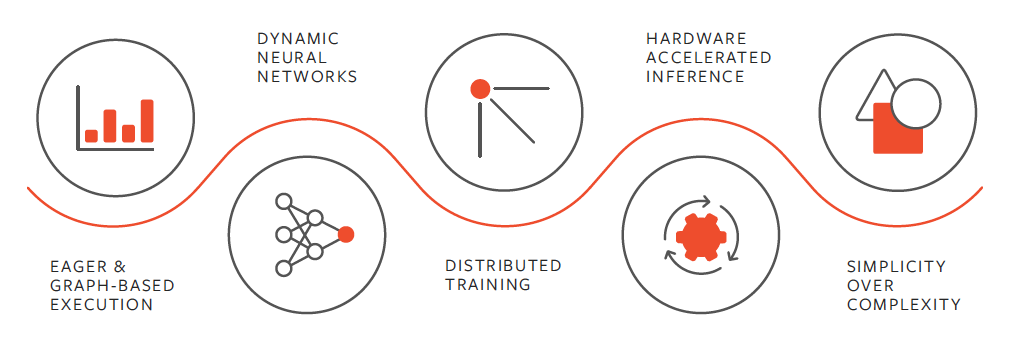
Among many others, all of these tools help in the process of tensor computation, or neural network creation and training. PyTorch also comes with the huge benefit of dynamic neural networks that can be accelerated on GPUs, giving us massive performance gains across most, if not all ML tasks.

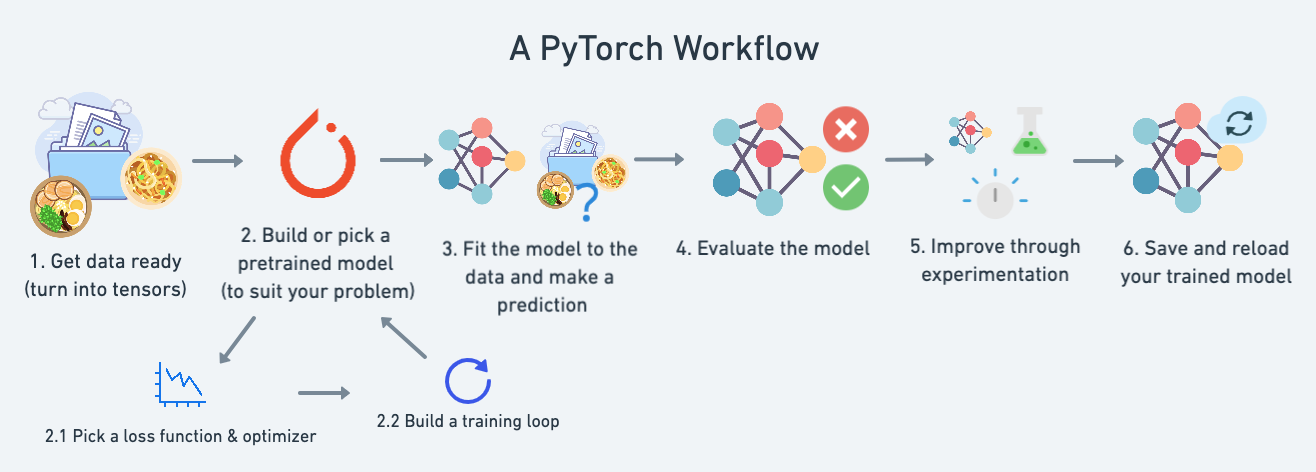
A Standard PyTorch Workflow

A typical PyTorch workflow has a structure which goes from your data to building a model which can properly represent that data, and finally creating a training loop and iterating upon the model until it fits your data.

PyTorch's Core Concepts

While the PyTorch docs are quite extensive, there are a few core concepts that everything else is built upon, which makes approaching this framework for the sake of curiosity or experimentation much less daunting.

Tensors

Tensors are the fundamental data structure in PyTorch: multi-dimensional arrays similar to NumPy arrays that can be used on GPUs to accelerate computation. In order to better understand Tensors, I HIGHLY recommend people watch this video by Dan Fleisch called What's a Tensor?; It is a very easy-to-follow explanation, with a great breakdown for some intuition.

From a simple understanding, we can break things down into a few more familiar concepts:

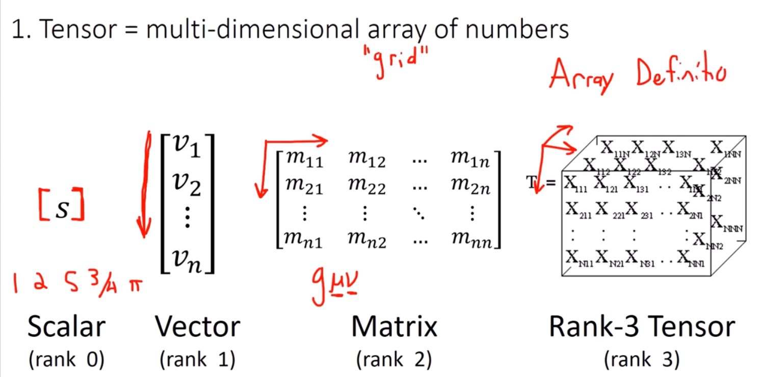
1. Scalars, Vectors, and Matrices:

• Scalar: A single number, or a 0-dimensional tensor. Think of it as a lone data point.
• Vector: A 1-dimensional tensor, like a list of numbers or a single row/column in a spreadsheet.
• Matrix: A 2-dimensional tensor, akin to a grid of numbers, much like a table or a spreadsheet.

2. Higher-Dimensional Data - Tensors:

• Rank-3 Tensor: Imagine a cube filled with numbers. This is a 3-dimensional tensor.
• Beyond: Tensors can have even higher dimensions (PyTorch has an N-Dimensional Tensor implementation), though this becomes increasingly hard to visualize.

Please note that “this is a seriously limited and oversimplified definition” of a tensor. I'd recommend at least watching part of the video mentioned above, Dan Fleisch - What's a Tensor?, for a better overview.

I mentioned that PyTorch implements N-Dimensional Tensors; What this means is that a Tensor can have as many dimensions as necessary in order to appropriately model provided data.

With all of this being said, creating a tensor with PyTorch can be very simple:

import torch

x = torch.randn(3, 4)  # random 3x4 tensor

If we print x, we can see the raw values which were added to our tensor, like so:

Autograd

Autograd is PyTorch's automatic differentiation engine. It's a feature that makes training neural networks not just possible, but efficient. What does Autograd actually do? In essence, it tracks all the operations that are performed on tensors, and it builds a computational graph on the fly, behind the scenes. This graph is then used to compute gradients, which is how the model finds the optimal values necessary to fit our data distributions.

Put simply: Autograd helps calculate how each parameter needs to change to improve your model's prediction accuracy. This process is known as backpropagation.

The computational graph is created dynamically during the execution of your code, which allows you to change your model's architecture or operations, and Autograd will adapt seamlessly- a big advantage for quick experimentation.

Inside of Google Colab, I've put together a basic example of how gradients get updated thanks to Autograd:

1. Make a Tensor: We create a tensor x with requires_grad=True, which tells Autograd to track operations on this tensor.
2. Perform Operation: We then perform some operation, saving the results to a new variable z, and we call backward() on z to compute the gradients.
3. Display Gradients: The result is stored in x.grad; Printing this gives us the gradient of z with respect to x.

torch.nn

When it comes to actually constructing the layers for our neural networks, PyTorch provides the nn module. torch.nn is a robust framework for constructing and managing layers and operations within our model, simplifying the process of defining our model's architecture. At the heart of this module is nn.Module, which acts as a blueprint for you to use when creating your own models.

nn.Module is a base class that you can subclass to define your neural network architecture. It handles a lot of the boilerplate for you, such as parameter initialization and forward pass execution. This makes it easier to focus on the design of your network without getting bogged down by too many details.

To give us a clearer picture, let's look at a simple example of a two-layer Multi-Layer Perceptron (MLP) using the nn.Module API:

import torch.nn as nn

class MLP(nn.Module):
    def __init__(self, input_size, hidden_size, output_size):
        super().__init__()
        self.hidden = nn.Linear(input_size, hidden_size)
        self.output = nn.Linear(hidden_size, output_size)
      
    def forward(self, x):
        x = torch.relu(self.hidden(x))
        x = self.output(x)
        return x

In our class, that inherits from nn.Module, we set up the layers of the network: one hidden layer and one output layer (which are both linear transformations) in our constructor. The forward method is our forward pass, where we apply a ReLU activation function (torch.relu) to the hidden layer's output.

Subclasses of nn.Module can contain any number of layers and operations, and you can nest nn.Module subclasses to create very complex architectures. This modularity is one of PyTorch's strengths, allowing you to build sophisticated models by combining simple components in a pythonic way.

Optimizers

Optimizers play a role in updating the model's parameters to minimize the loss function. PyTorch offers a comprehensive suite of optimization algorithms through its torch.optim module, each tailored to different types of models and training scenarios.

Optimizers work by adjusting the weights of your model based on the computed gradients, which are provided by Autograd. The choice of optimizer can significantly impact the speed and quality of your model's convergence, making it an important consideration in your training loop's setup.

One of the most popular optimizers is Adam, which stands for Adaptive Moment Estimation. It's known for its efficiency and performance across a wide range of tasks, thanks to its ability to adapt the learning rate for each parameter dynamically throughout the model's training process.

Here's a quick example of how we can set up the Adam optimizer for our simple MLP model:

import torch.optim as optim

model = MLP(10, 100, 2)  
optimizer = optim.Adam(model.parameters(), lr=1e-3)

Related: See Machine Learning Mastery's - "Understanding the Dynamics of Learning Rate on Deep Learning Neural Networks" for an in-depth breakdown of learning rates.

The torch.optim module includes other optimizers like SGD (Stochastic Gradient Descent), RMSprop, and more; Each of these optimizers has its own strengths and applicable scenarios. Choosing the right optimizer often involves experimentation, and will depend on factors such as the complexity of your model, the size of your dataset, and the specific problem you're tackling.

Data Loaders

PyTorch's torch.utils.data module provides tools to handle datasets and create iterable data loaders. This is especially useful for managing large datasets and ensuring efficient data shuffling and batching.

Here's a simple example, using some randomly generated data, of how you could create a data loader. Here, we will use PyTorch's built-in dataset class and data loader functionality:

import torch
from torch.utils.data import DataLoader, TensorDataset

X = torch.randn(1000, 10)
y = torch.randint(0, 2, (1000,))

dataset = TensorDataset(X, y)
train_loader = DataLoader(dataset, batch_size=32, shuffle=True)

for x_batch, y_batch in train_loader:
    print(x_batch.shape, y_batch.shape)
    break

1. Example Data: Here, X is a tensor containing 1000 samples, each with 10 features. y is a tensor of 1000 binary labels.
2. TensorDataset: The TensorDataset wraps the feature tensor X and label tensor y together, making it easy to access both inputs and targets simultaneously.
3. DataLoader: The DataLoader takes the dataset and provides an iterable over the data, where batch_size=32 specifies that each batch contains 32 samples. The shuffle=True option ensures the data is shuffled at the start of each epoch.
4. Batch Processing in Training Loop: In the training loop, for x_batch, y_batch in train_loader iterates over the data loader, yielding batches of x_batch (features) and y_batch (labels) that are used in the forward and backward passes.

By using TensorDataset and DataLoader, PyTorch abstracts away much of the complexity involved in data handling, providing a straightforward interface for iterating over our batches of data. Because of this, we can focus much more on optimizing and improving our model's performance, rather than worry too much about handling everything ourselves.

Putting it All Together

Making a PyTorch Training Loop

Now that we've gone over the core concepts of PyTorch, we can begin to see how they fit together in a simple training loop. This is where all of the magic happens, and where we transform raw data into a trained model ready to make predictions on new data.

What a Training Loop Does

Here's a quick breakdown of what a PyTorch training loop involves:

1. Define your model using nn.Module: Start by setting up your neural network architecture. This involves creating a class that subclasses nn.Module and defines the layers of your model, as well as what operations your model can perform.

class MLP(nn.Module):
    def __init__(self, input_size, hidden_size, output_size):
        super().__init__()
        self.hidden = nn.Linear(input_size, hidden_size)
        self.output = nn.Linear(hidden_size, output_size)
      
    def forward(self, x):
        x = torch.relu(self.hidden(x))
        x = self.output(x)
        return x

2. Specify a loss function and optimizer: Choose a loss function that quantifies how well your model is performing, like nn.CrossEntropyLoss for classification tasks. Then, select an optimizer from torch.optim to update your model's parameters based on the computed gradients.

model = MLP(10, 100, 2)  
optimizer = optim.Adam(model.parameters(), lr=1e-3)

3. Iterate over training data: Use a data loader to feed batches of data into your model. This helps in managing memory efficiently and speeds up the training process.

   1. See the Data Loader section above for a brief explanation and example code snippet.
   2. Read more about Datasets & DataLoaders from the PyTorch Docs.

4. For each batch from our data:

   • Perform a forward pass to compute predictions: Pass your input data through the model to get predictions.
   • Calculate the loss: Use the loss function to measure how far off the predictions are from the actual labels.
   • Perform a backward pass to compute gradients: Call backward() on the loss to compute the gradients of the loss with respect to the model's parameters.
   • Update model parameters with the optimizer: Use the optimizer to adjust the parameters in the direction that reduces the loss.

5. Rinse and repeat: Just like that, we continue this process for a specified number of epochs, or until your model reaches an acceptable level of performance.

Training Loop - Code Example

import torch
import torch.nn as nn
import torch.optim as optim

model = MLP(10, 100, 2)

criterion = nn.CrossEntropyLoss() # loss
optimizer = optim.Adam(model.parameters())

for epoch in range(100):
    for x_batch, y_batch in train_loader:

        y_pred = model(x_batch)
        loss = criterion(y_pred, y_batch)
        
        optimizer.zero_grad()
        loss.backward()
        optimizer.step()

From the code sample above, we illustrate all of the steps involved in a simple PyTorch training loop, which facilitates our ability to train models on our own data:

1. Import Libraries: Lines 1-3 import the necessary PyTorch libraries for building and training models.
2. Define the Model: We initialize the MLP model with specified input, hidden, and output sizes, using model = MLP(10, 100, 2).
3. Define Loss Function and Optimizer: Next, we set up the loss function to use (nn.CrossEntropyLoss) and the optimizer with optim.Adam(model.parameters()).
4. Training Loop: We use a for loop to go over a specified number of epochs (epoch in range(100)), repeating our operations as many times as declared.
5. Data Loading: Inside of our training loop, we use another for loop which iterates over the batches of data provided by our data loader, train_loader. See the Data Loaders section and example snippet for more on how this is handled.
6. Forward Pass and Loss Calculation: Compute the model's predictions (model(x_batch)), and calculate the loss for the current batch (criterion(y_pred, y_batch)).
7. Backward Pass and Parameter Update: Finally, we clear old gradients by dropping them to 0 (optimizer.zero_grad()), compute new gradients with loss.backward(), and update the model's parameters with optimizer.step().

Related Note: If you find yourself still wondering about the difference between a batch (dealing with our data), and an "epoch". Here's another great article by Machine Learning Mastery that breaks this down!

Conclusion

In this post, we have only scratched the surface of the fundamental components of PyTorch. I've shown how basic concepts can come together to form a simple training loop. We've seen how PyTorch's intuitive design makes deep learning both accessible and efficient. It empowers researchers and hobbyist developers alike, letting us use powerful modern deep learning techniques.

Just a Training Loop

Our exploration here has focused solely on a simple PyTorch training loop, using throwaway data. Training loops are only one stage of model development; An equally important step in creating a good model is testing / validating your model's predictions, ensuring that your model generalizes well to unseen data. In a future post, I intend to go over the creation of a testing loop, and will write more about how to evaluate model performance, allowing you to iterate on everything and create even better models, i.e. make more accurate predictions.

If you've made it this far, thank you for reading. I hope everyone had a great New Year.

// January 5th, 2025